Maths behind Bayesian Duration Calculator
Written by Anshul Gupta
Introduction
The culture of experimentation is strongly picking up in several sectors of industry. It has become imperative to measure the impact of product ideas with an A/B test. But before one experiment, it is highly recommended to calculate the sample size needed to measure the effect. This advice comes from the traditional approach of hypothesis testing(used in clinical trials, agriculture, etc) as it gives an estimate of the experiment cost one is likely to incur. Running a test beyond the necessary threshold when the desired effect doesn’t exist can result in wasted time and resources that could be spent elsewhere. That is why this calculation is so important.
Overview
The duration calculators available in the industry are built on the frequentist based hypothesis testing in which for a certain Type 1 and Type 2 error and a given Conversion Rate(CR), improvement, and number of variations one gets an estimated sample size (refer A/B Test Duration Calculator for more details). However, if one cares about bayesian metrics these calculators do not provide a correct estimate of the test as they do not take into account the bayesian metrics criteria in their sample size calculation.
We at VWO have built a sample size calculator that aligns well with the bayesian metrics we use to check smart decisions in an A/B test. This gives the user a perspective on when a test will end with a smart decision in VWO in median cases if the assumptions on conversion rate and minimum improvement of an experiment by the user holds true.
We also provide a heuristic to obtain extreme estimates beyond which there is no point running the test for a given improvement. Traditionally this requires simulations at the bayesian metric level which was computationally intensive and used to take a lot of time to finish. Now using the proposed analytical form, the simulations required to obtain extreme estimates can be performed blazingly fast.
In the proposed bayesian calculator you are asked for the base conversion rate, the number of variations you plan to have, the size of the minimum improvement you wish to test in the experiment, and the metric threshold. The result of the calculation is the size of the samples needed to reach the threshold.
We use probability to beat baseline and Potential Loss metrics to measure statistical significance. To learn more about their definitions please visit - How VWO Calculates a Winning Variation.
Estimating Visitors for probability to beat baseline
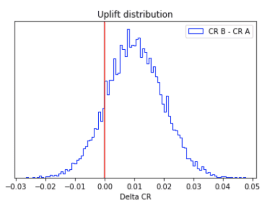
The probability to beat baseline(PBB) is the number of times a Variation is better than the other variation after Monte Carlo sampling is performed. Another way to look at it graphically when two variations are involved, if we compute an uplift distribution such that the difference in Monte Carlo samples of B from A, where Conversion Rate of Variation B is better than Conversion Rate of A we would obtain the following plot as:
- the
PBBof B can be interpreted as the area under the uplift curve and the right of the y-axis - and, the
PBBof A would be the area under the uplift curve and on the left of the y-axis.
To estimate the number of visitors to see improvement in B we will try to find the standard deviation of uplift distribution(Standard Error) such that:
$$PBB_B \approx PBB_{Threshold}$$
Then by using the standard error and standard deviation obtained from input parameters we can obtain a visitor estimation.
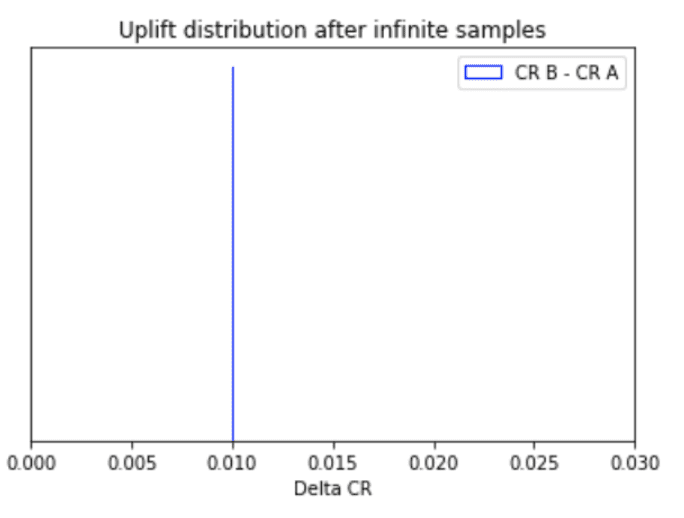
Though we don’t know the analytical form of uplift distribution, however, as per the Central Limit Theorem, after a certain number of visitors, the uplift distribution tends to become Normal Distribution whose mean is:
$$\delta(CR * Improvement)$$
and Standard Deviation would depend upon the number of visitors obtained in the test. Theoretically, if infinite data is provided it would become Dirac Delta distribution.
Based on the assumption of uplift distribution as Normal distribution, PBB can be computed analytically as:
$$1 - Norm(\delta,SE).cdf(0)$$
where CDF is the cumulative density function and SE is the standard error.
The standard deviation of the data distribution can be computed as:
$$\sigma_1^2 = CR1(1-CR1)$$ $$\sigma_2^2 = CR2(1-CR2)$$ $$\sigma = \sqrt{\sigma_1^2 + \sigma_2^2}$$
Using Standard Error(SE) and σ, we can compute the Number of Visitors(N) as:
$$N = nVars * \Big( \dfrac{\sigma}{SE} \Big) ^2$$
where nVars is the Number of Variations
Estimating Visitors for Potential Loss
A potential loss is a distribution that can be interpreted as the loss in conversion rate you are likely to incur if you select a variation that is not the best variation. Logic to compute the potential loss is:
$$Potential Loss_B = Max(0, CR_{Not\space B} - CR_B)$$
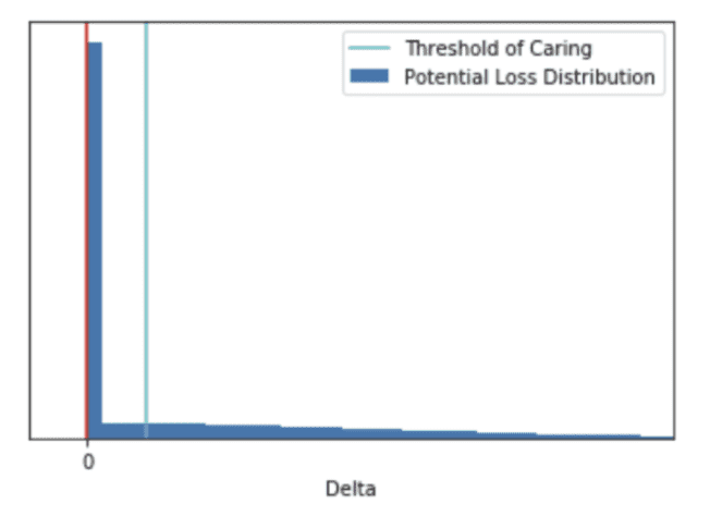
Essentially, it is an uplift distribution where the probabilities associated with the negative values of uplift are concentrated at 0. The resultant distribution of variation B would be similar to the following plot.
We will find the standard deviation of this distribution such that its mean becomes close to the threshold of caring. Then by using the standard error and standard deviation obtained from input parameters we can obtain a visitor estimation as explained in the previous section. We will use a Truncated Normal Distribution with range [low, high] to represent the positive non-zero portion of the above distribution whose analytical mean can be computed as:
$$\mu_{uplift} = -\delta$$ $$\sigma = SE$$ $$a = \dfrac{low-\mu_{uplift}}{\sigma}$$ $$b = \dfrac{upper-\mu_{uplift}}{\sigma}$$ $$\mu = truncNorm(\mu_{uplift}, \sigma, a, b).mean()$$
Then we’ll adjust the mean by taking into account the probability of 0 as represented in the above plot as
$$\mu_{adjusted} = \mu * (1 - Norm(\mu_{uplift},\sigma).cdf(0))$$
Estimating standard error
We'll perform a binary search on standard error such that it provides an estimate close to the required probability to beat baseline/Potential Loss within a certain error bound.
Duration estimation in extreme cases
We perform several simulations to obtain a distribution of estimation using the following algorithm to get an estimate in extreme cases like 90/95 percentile
- Estimate number of visitors using input
CR, improvement, number of variations, and the required threshold using analytical equations. - Based on the estimated visitors per variation as the number of trials, perform Bernoulli trials, and obtain new conversion rate and improvement.
- Using the new conversion rate and improvement obtain an estimate of visitors using the analytical equation.
- Perform 2 and 3, 1000 times to obtain an estimated visitor distribution.
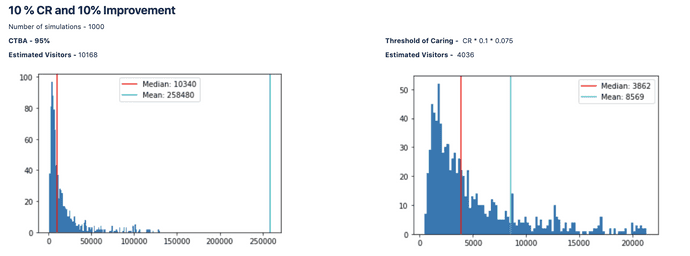
Simulation Results
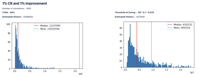
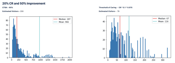
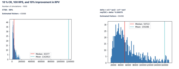
Notice how close the median of estimates from 1000 simulations is to the visitor estimate obtained from the analytical equation.
Duration Calculator Revenue
We have built the duration calculator for revenue using the same principles described above. The only difference would come in the computation of the standard deviation of the data distribution. We will use the following analytical form of the standard deviation:
$$\sigma^2 = CR * \sigma_Z^2 + CR*(1-CR)*\mu_Z^2$$
Z is a random variable used to represent revenue per sale distribution.
Simulation Results
Summary
Sample Size calculators can prove to be very helpful in planning the time and resources to invest in a statistical test. The analytical form of equations proposed in this blog provides a general framework to obtain duration estimation for any parametric model used to measure the effect in an A/B test.
This is just one way that we are improving the experimentation experience at VWO. As the next steps, we plan to integrate it with the VWO app to obtain more realistic estimates in a test while it is running.

